Multi-Teacher On-Policy Distillation

最近小米开源了新模型Mimo-v2-flash的技术报告，其中提出的Multi-Teacher On-Policy Distillation感觉有点业务价值，能够将多个teacher model的能力蒸馏到一个模型上，同时减少模型之间的性能差异。

Overview of Post-Training Pipeline

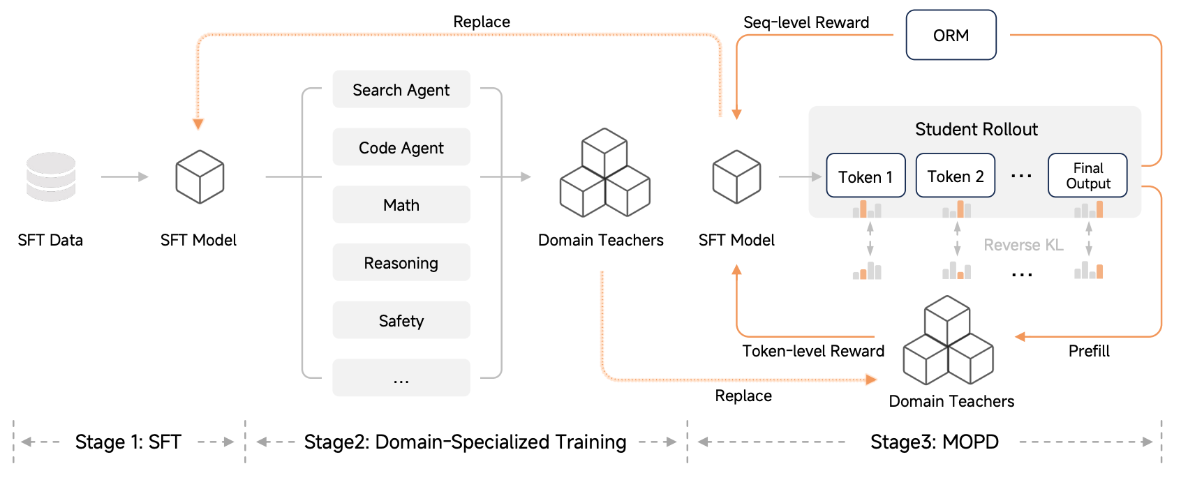
default name — 图1: Overview of MiMo-V2-Flash post-training stages.

Stage1: Supervised Fine-Tuning

实现一个基础的指令遵循版本模型

Stage2: Domain-Specialized Training

基于RL训练一系列领域专家模型，这其中包含了agentic的专家(search, coding, general tool use)和non-agentic的专家(mathematical reasoning, general reasoning, safety alignment)，每个专家模型都在领域内取得较高性能。

Stage3: Multi-Teacher On-Policy Distillation

定义学生策略为$\pi_\theta$，定义学生采样策略$\mu_\theta$，定义$\pi_{dx}$为prompt $x$对应的领域专家。学生策略和专家策略之间的reverse KL散度定义为：

$$ \mathcal L_{\text{reverse-KL}(\theta)}=-\mathbb E_{x\sim\mathcal D,y_t\sim\pi_\theta(\cdot\vert x,y_{< t})}\log\frac{\pi_{dx}(y_t\vert x,y_{< t})}{\pi_\theta(y_t\vert x,y_{<t})} $$

简化一下：

$$ J(\theta)=\mathcal L_{\text{reverse-KL}}(\theta)=-\mathbb E_{y\sim\pi_\theta}\left[\log\frac{\pi_{\text{Teacher}}(y)}{\pi_\theta(y)}\right] $$

对于离散的文本生成，该期望就是把所有可能的句子$y$遍历一遍：

$$ J(\theta)=-\sum_y\pi_\theta(y)\cdot(\log\pi_{\text{Teacher}}(y)-\log\pi_\theta(y)) $$

接下来对$\theta$求梯度：

$$ \nabla_\theta J(\theta)=-\sum_y\left[\nabla_\theta\pi_\theta(y)\cdot(\log\frac{\pi_{\text{Teacher}}}{\pi_\theta})+\pi_\theta(y)\cdot\nabla_\theta(\log\frac{\pi_{\text{Teacher}}}{\pi_\theta})\right] $$

对于梯度的第二部分：

$$ \text{Part2}=\pi_\theta(y)\cdot\nabla_\theta(\log\pi_{\text{Teacher}}-\log\pi_\theta(y)) $$

由于Teacher固定，$\nabla_\theta\log\pi_{\text{Teacher}}=0$，接着剩下$\sum_y\pi_\theta(y)\nabla_\theta\log\pi_\theta(y)$，很明显，通过对数导数转换，该项为0:

$$ \sum_y\pi_\theta(y)\nabla_\theta\log\pi_\theta(y)=\sum_y\nabla_\theta\pi_\theta(y)=\nabla_\theta\sum_y\pi_\theta(y)=\nabla_\theta 1=0 $$

因此最终$J(\theta)$的梯度为：

$$ \nabla_\theta J(\theta)=-\sum_y\nabla_\theta\pi_\theta(y)\cdot\left(\log\frac{\pi_{\text{Teacher}}}{\pi_\theta}\right) $$

接下来，基于$\nabla\pi_\theta=\pi_\theta\cdot\nabla\log\pi_\theta$恒等式，$J(\theta)$的梯度变为：

$$ \nabla_\theta J(\theta)=-\sum_y\pi_\theta(y)\cdot\nabla_\theta\log\pi_\theta(y)\cdot\left(\log\frac{\pi_{\text{Teacher}}}{\pi_\theta}\right) $$

将求和重新写回期望的形式，得到：

$$ \nabla_\theta J(\theta)=-\mathbb E_{y\sim\pi_\theta}\left[\left(\log\frac{\pi_{\text{Teacher}}}{\pi_\theta}\right)\cdot\nabla_\theta\log\pi_\theta(y)\right] $$

会发现这里已经和策略梯度很像了。目前的公式假设数据$y$是从当前模型$\pi_\theta$采样出来的，实际上，往往使用一个略微不同的策略$\mu_\theta$（旧版本），因此这里需要用重要性采样进行修正：

$$ \mathbb E_{y\sim\pi_\theta}[f(y)]=\mathbb E_{y\sim\mu_\theta}\left[\frac{\pi_\theta(y)}{\mu_\theta(y)}\cdot f(y)\right] $$

把这个应用到$J(\theta)$梯度上，梯度变成了：

$$ \nabla_\theta J\approx-\mathbb E_{y\sim\mu_\theta}\left[\frac{\pi_\theta}{\mu_\theta}\cdot\left(\log\frac{\pi_{\text{Teacher}}}{\pi_\theta}\right)\cdot\nabla_\theta\log\pi_\theta\right] $$

由于原始目标逆向KL在LLM中是离散的，涉及采样，没法直接作为损失反向回传梯度。我们需要找到一个损失函数，让它的梯度刚好等于我们上面计算出来的近似梯度，同时梯度回传不受阻碍。观察梯度结构可以发现：

$$ \text{Gradient}=\text{Coefficient}\times\nabla_\theta\log\pi_\theta $$

实际上，$\text{Coefficient}$也带$\theta$，这里作者直接选择冻结这部分，使之不可回传梯度，通过引入stop_gradient(sg)实现，sg(x)的定义（在pytorch里等价于x.detach()）：

$$ \begin{cases} \text{sg}(x)=x, & \text{forward pass} \\ \frac{\partial\text{sg}(x)}{\partial x}=0, & \text{backward pass} \end{cases} $$

这里是一个逆向工程，从理想梯度的公式形式上$\nabla J=\mathbb E[A\cdot B\cdot\nabla\log\pi]$，可以定义损失函数为$L=C\cdot\log\pi$，那么它的导数是：

$$ \nabla L=(\nabla C)\cdot\log\pi+C\cdot(\nabla\log\pi) $$

而我们需要的结果仅仅是$C\cdot(\nabla\log\pi)$，因此我们必须强行让第一项$(\nabla C)\cdot\log\pi$消失，也就是$\nabla C=0$，所以直接将系数常量化就可以得到理想损失。

最终，直接对$\text{Gradient}$积分可以得到最终损失函数形式：

$$ \mathcal L_{MOPD}=-\mathbb E_{y\sim\mu_\theta}\left[\text{sg}\left(\frac{\pi_\theta}{\mu_\theta}\cdot\log\frac{\pi_{\text{Teacher}}}{\pi_\theta}\right)\cdot\log\pi_\theta\right] $$

在此基础上，为了防止当前策略和采样策略差别太大，对重要性采样系数做了限制：

$$ \omega(\theta)=\begin{cases} \text{sg}[\frac{\pi_\theta}{\mu_\theta}],&\epsilon_{\text{low}}\le\frac{\pi_\theta}{\mu_\theta}\le\epsilon_{\text{high}}, \\ 0,&\text{other}, \end{cases} $$

此外，作者对于一个完整的采样的损失计算，加入了对采样y长度的归一化处理：

$$ \mathcal L_{MOPD}=-\mathbb E_{x\sim\mathcal D,y\sim\mu_\theta(\cdot\vert x)}\left[\frac{1}{\vert y\vert}\sum_{t=1}^{\vert y\vert}\omega_t\cdot\hat A_{MOPD,t}\cdot\log\pi_\theta(y_t\vert x, y_{< t})\right] $$

其中：

$$ w_t(\theta) = \begin{cases} \text{sg} \left[ \frac{\pi_\theta(y_t | x, y_{<t})}{\mu_\theta(y_t | x, y_{<t})} \right], & \epsilon_{\text{low}} \leq \frac{\pi_\theta(y_t | x, y_{<t})}{\mu_\theta(y_t | x, y_{<t})} \leq \epsilon_{\text{high}}, \\ 0, & \text{other}, \end{cases} $$

$$ \hat A_{MODP,t}=\text{sg}\left[\log\frac{\pi_{\text{Teacher}}(y_t\vert x,y_{<t})}{\pi_\theta(y_t\vert x,y_{< t})}\right] $$

最后写一个简单的pytorch实现

 1
 2
 3
 4
 5
 6
 7
 8
 9
10
11
12
13
14
15
16
17
18
19


import torch
import torch.nn.functional as F

def compute_mopd_loss(policy_logits, sampling_logits, teacher_logits, input_ids, eps_low, eps_high):
    pi_log_all = F.log_softmax(policy_logits, dim=-1) # [B, S, V]
    mu_log_all = F.log_softmax(sampling_logits, dim=-1) # [B, S, V]
    te_log_all = F.log_softmax(teacher_logits, dim=-1) # [B, S, V]

    pi_log = pi_log_all.gather(-1, input_ids.unsqueeze(-1)).squeeze(-1) # [B, S]
    mu_log = mu_log_all.gather(-1, input_ids.unsqueeze(-1)).squeeze(-1) # [B, S]
    te_log = te_log_all.gather(-1, input_ids.unsqueeze(-1)).squeeze(-1) # [B, S]

    ratio = torch.exp(pi_log - mu_log) # [B, S]
    mask = (ratio >= eps_low) & (ratio <= eps_high) # [B, S]
    w_t = torch.where(mask, ratio, torch.zeros_like(ratio)).detach() # [B, S]
    adv = (te_log - pi_log).detach() # [B, S]
    token_loss = - (w_t * adv * pi_log) # [B, S]
    
    return token_loss.mean()

PPO or MOPD

粗浅理解一下PPO和MOPD的关系（在LLM场景下）

对于PPO，从策略梯度出发：

$$ \nabla_\theta J(\theta)=\mathbb E_{y\sim\pi_\theta}[\nabla_\theta\log\pi_\theta(y)\cdot\hat A] $$

经过重要性采样，得到：

$$ \nabla_\theta J(\theta)=\mathbb E_{y\sim\mu_\theta}\left[\frac{\pi_\theta(y)}{\mu_\theta(y)}\cdot\hat A\cdot\nabla_\theta\log\pi_\theta(y)\right] $$

这里，PPO没有sg化$\frac{\pi_\theta(y)}{\mu_\theta(y)}$，只是sg化了$\hat A$，接着直接基于$\nabla_\theta\pi_\theta=\pi_\theta\nabla_\theta\log\pi_\theta$，得到损失函数，之后再做clip处理：

$$ \mathcal L_{PPO}=\mathbb E_{y\sim\mu_\theta}\left[\frac{\pi_\theta(y)}{\mu_\theta(y)}\cdot\text{sg}(\hat A)\right] $$

而对于MOPD，可以理解成直接把Teacher模型作为PPO中的Critic模型，基于Teacher模型的概率分布得到优势，与此同时，为了让策略模型学习到Teacher模型的知识，而不是从策略本身变化的角度出发，把ratio和advantage全部sg化，只要Teacher模型的概率高于策略模型，就鼓励策略模型提高该动作的概率。

Reference

[1] Luo et al. “MiMo-V2-Flash Technical Report” Xiaomi, 2025.

Overview of Post-Training Pipeline#

Stage1: Supervised Fine-Tuning#

Stage2: Domain-Specialized Training#

Stage3: Multi-Teacher On-Policy Distillation#

PPO or MOPD#

Reference#